
Andy Schofield (University of Birmingham, UK)
 Quantum Criticality - A tutorial
Blogged by Michael Norman and Piers Coleman
Andy is going to do a blackboard talk so let's see how good my eyesight is. The focus will be on ZrZn2, a weak ferromagnet, with the emphasis of how current-current interactions affect metals, and whether the standard Hertz-Millis theory (time dependent Ginzburg-Landau) works or not.
To motivate all of this, let us consider a few cases first. The "strange metal" behavior of cuprates exhibits linear T resistivity over a wide range of temperatures, but the nature of the "ordered" (pseudogap) phase is controversial. CePd2Si2 is an antiferromaget, which is suppressed to zero under pressure. Near the resulting quantum critical point, one sees unconventional superconductivity. Or consider a first order transition (like liquid-gas). At the end of the first order line, one has a second order critical end point, which in principle could be tuned to zero by varying some quantity like field, pressure, or what have you.
Q: What do you mean by critical fluctuations?
AS: Near the ordering phase line, small variations of the order parameter field lead to large responses.
 In ZrZn2, the electrical resistivity varies as T^5/3. The thermal resistivity instead varies as T. This is seen in nickel doped palladium as well, where Ni doping drives paramagnetic Pd into a ferromagnetic state. The phase line varies as (x-xc)^3/4, where xc is the concentration of Ni that first induces ferromagnetism. In Ni doped Pd, the specific head coefficient C/T varies as the log of T.
Now to the tutorial. In Landau theory, there is a one to one mapping between non-interacting electrons and fermionic quasiparticles. One can characterize the system by a distribution function, n(E), which varies with momentum, k. The difference from the Fermi function is determined by interactions. This can be determined by a scattering rate, which can be calculated using Fermi's golden rule, taking into account the presence of a filled Fermi sea. One finds that the scattering rate depends on omega^2, where omega is the energy loss. Including temperature, omega^2 changes to omega^2 + (pi*T)^2.
This is a phase space argument. Now, let's assume the scattering potential depends on momentum and energy. Exploiting energy and momentum conservation, one sees that the transferred energy, omega, is restricted to being (T=0) between zero and the energy E of the state, whereas the transferred momentum is restricted to being between omega/vF and 2kF, where vF is the Fermi velocity and kF is the Fermi momentum. The result for the scattering rate (easily derived by power counting) is
1/tau ~ Integral(0 to E) omega domega Integral (omega/vF to 2kF) q^(D-3) dq |V(q,omega)|^2 where V is the scattering potential and D the dimensionality. If V is constant, in D=3, this gives E^2 as before, whereas in D=2, one gets E^2log(E) instead.
If V has structure, then one gets something more interesting. Coulomb scattering looks promising, since V ~ 1/q^2, but screening converts this to 1/(q^2 + qTF^2) where qTF is the Thomas-Fermi wavevector, and the infrared divergence is cutoff.
On the other hand, magnetic scattering is not screened, so this is more promising. Assuming an Amperean potential between currents, j. Using Maxwell equations and Ohm's law, the current-current scattering potential varies as 1/(q^2 - omega^2/c^2 + i*omega*sigma) where sigma is the conductivity. The last term in the denominator is the so-called skin effect. In the clean limit, sigma varies as 1/q. So V^2 goes as 1/q^4 down to q of order omega^(1/3). The result is that 1/tau (D=3) now goes like E instead of E^2. Since 1/tau is a measure of the imaginary part of the self-energy, by Kramers-Kronig, one can show that the real part of the self-energy goes as E*log(E). Therefore, the specific heat coefficient goes as log(T).
But the problem is that the ratio of the Amperean potential to the Coulomb one goes as vF^2/c^2, which is of order 10^(-6). So, although one does indeed find a breakdown of Fermi liquid theory, this only shows up at extremely low temperatures.
Q: This looks like a classical treatment?
AS: Yes and no. One has a Fermi surface, and then treats things in a semi-classical approximation.

Part II. Andy begins with a summary of the first lecture. The blackboard is empty and we are ready for another wonderful blackboard talk. Andy is going to use the results from the last lecture to gain insight into the magnet quantum critical point. Andy says - if I think about an electric current and imagine how it is affected by small angle scattering. A quasiparticle receives a tiny knock, and is now diverted through a small angle - this contributes to the decay rate of the quasiparticle, but it does not affect the transport current very much. (Bloggers aside: We saw this yesterday in Lara Benfatto's talk - this is the effect of the vertex corrections. ) The change in the current is
Delta j = k_F (1-cos (theta)) ~ k_F * (q/k_F)^2
which is reduced by the factor q^2s, so that transport rate is now
current decay rate = Integral omega domega Integral d^D-1 q dq/ q^2 * |V(q,omega)|^2
* additional q^2 term
The q^D-1 cancels with q^2 in D=3, the |V(q,omega)|^2 ~ 1/q^4 at q^2 > omega/q, so the lower limit becomes omega^1/3, so when we do it, we have dq/q^2 from omega^1/3 , which gives 1/omega^1/3 from the q-integral, which gives in the end, with the frequency integral omega^5/3 -> T^5/3. (Blogger's aside - this result is consistent with simple dimensional analysis! AS answers that it is good to see how this works in detail. )
Q: wouldn't you have to do this self-consistently, because the resistivity appears in the damping rate?
AS: Potentially - but it comes back to whether the effective mass should be calculated self-consistently. But the answer seems to be, it doesn't affect anything.
AS asks - can we use these results for U(1) gauge theories, where the coupling constant is much bigger. AS reminds us about the method that was used by Yong Baek in his talk on spin liquids -
fermion = spinon creation * holon (slave boson approach)
Now this introduces a local gauge invariance, and to make this work once the spinons are delocalized, you need a fictitious electromagnetism.
Q: Is this really fictitious - after all it leads to a collective " artificial light ",
AS: I wanted to make the point that it is not conventional Electromagnetism. It is observable, because it will lead to a T^2/3 specific heat. Andy points out that the energy will go like
T^2/3. (Blogger didn't quite catch it all).
Now we discuss Matter close to quantum criticality. The action is written down
S = phi[ r0 + q^2 + |omega|/Gamma(q)]phi + u phi^4
Why do I have a term proportional to omega? Answer - because this is allowing for the physics of damping?
quasiparticle interacts with medium that is almost magnetic, and it sends out modes with a propagator that is the inverse of the quadratic coefficient of S
1 / [r0 + q^2 + |omega|/Gamma(q)]
If you were in an insulator, the damping would be replaced by omega^2. But here we have a metallic environment, the magnon interacts with the Fermi sea which makes particle-hole pairs.
Q: can this be derived?
AS: Yes, but we now know there are some problems with the derivation (non-analytic terms in frequency for example).
So in a system like ZrZn_2 close to criticality, the propagator of the critical magnetization is essentially identical with the current-current fluctuations we talked about this morning, but with a much stronger coupling. And we see a T^5/3 resistivity as expected. Note that the thermal resistivity, which is just governed by the quasiparticle relaxation rate, is still linear in T, as measured by Smith et al in the data shown below.
Q: how do you derive this from the partition function?
AS: Well - we'd like to rewrite the Boltzmann partition function in terms of states that are not eigenstates? Fortunately for me that question was answered long-ago by Feynman, who wanted to use position eigenstates in zero temperature qm. He showed that you could evalue the expectations of
<r | exp[-i H t] r'>
provided you split it up into tiny increments, and then sum over all "histories" {r(t)}. I'm trying to do exactly the same thing here,
< phi | exp[- H beta] |phi> = Sum over the {phi_j} configurations of
< phi | exp [ - H \delta \tau] |phi_1> x ..... x <phi_N-1| exp[-H \delta \tau |phi
I now have imaginary time, and I have to split it up into all trajectories of the magnetization in imaginary time.
Q: I understand all of this, but why does it give rise to the precise form in S that you have shown us?
AS: The answer is that this is the first allowable term in the expansion - why do I have a q^2 - the first that is allowed - you might have though omega^2, but because this is in a damped environment, you can have a |omega|. Actually what we have here is the Lindhardt function - a polarization bubble which has precisely this form.
 Q: But why do you have a 1/q in the damping omega/q.
AS: I kind of lied to you, because ferromagnet is an eigenstate. But when we look at long wavelength modes, (draws a wave) . In the FM, the decay rates are suppressed as the wavelength gets longer and longer, and this gives rise to a damping rate Gamma(q) ~ q. Balistic motion - the amount of time is proportional to the wavelength, which gives tau ~ lambda, 1/tau ~ q. But if it was a dirty ferromagnet, the electrons would diffuse, so now tau ~ lambda ^2, 1/ tau ~ q^2. Final thing I should mention is an antiferromagnet. Now it doesn't depend on the slight variations about the AFM wavelength, so damping rate is constant.
So for an antiferromagnet, the propagator becomes
1 / [ r0 + (Q-q)^2 + |omega|/Gamma_0]
where we expanding the Gamma around the afm wavevector. So now I can change my scattering rate formula, which now becomes centered around Q.
(Q-q) -> qtilde
The denominator has now gone away becomes big Q^2. The q^2/k_F^2 disappears because the scattering is now at large Q, which relaxes the current easily.
Q: Why don't you change the lower limits of integration in momentum?
AS: The upper cutoff isn't really important. Its kind of order (k_F). The lower cutoff is now when p^2 ~ omega, so lower limit is indeed changed to omega^(1/2)
But why is all of this wrong?
Well experimentally - in the FM - almost all of them become first order before we reach the QCP. (Bloggers aside, there is a new Yb system which does have a second order transition, but its more localized)
MnSi is a particularly fascinating case. It also doesn't go quantum critical - weakly first order - and worst, the power law, which is not actually T^5/3, but T^3/2, appears over a wide range of the tuning parameter (presssure) - and nobody understands this.
Theoretical reappraisal.
It turns out that there are additional terms in the LGW action. A more detailed analysis tells us that terms I've left out should affect the answer. Finally - almost everything I've discussed now applies to itinerant systems, where the magnetism is delocalized, but a lot of the crucial experiments are on f-electron systems where the magnetism is very localized, and the itinerant approach I've described here doesn't apply.
A better job of dealing with the FM QCP, there are non-analytic terms, eg in 3D, q^3/2 terms, which leads to fourth order terms that go negative, explaining why the transitions tend to go first order.
The current picture of the FM QCP is as follows:

Now the electrons are coupling to the transverse modes. The early pioneers did not quite take into effect the higher order transverse modes - but if you can gap them out by applying a field, you do get interesting quantum criticality at a metamagnetic QCP.
Puzzles in Heavy Fermion QCP.
Examples include CeCu6-xAu_x
The reason we thought things were fine - that we can ignore the mode-mode coupling terms can be ignored (above the upper critical dimension) - yet there is evidence that the system obeys E/T scaling - a result of something called "naive scaling" - which suggests that the underlying quantum critical point is somehow below its upper critical dimension. There is other evidence that the critical fluctuations are affecting all the Fermi surface - some kind of local quantum criticality.
Another example is YbRh2Si2, which has an incredibly low ordering temperature that is killed off by a tiny magnetic field. Seems to be an additional scale that is collapsing to zero T^* at the QCP. This is one of the great puzzles.
Ends with a cartoon about what might be going on. Conduction electron zooms past a spin and exchanges spin with it. The key question, is what is the fate of the localized spins. One side - the ordered state - they are localized - on the other hand, there is another possibility that the interaction between the electrons and the local moments could undergo a Kondo effect, whereby the electrons and local moments bind in delocalized heavy fermions.
An example of a delocalized heavy fermi liquid, Andy gives UPt3, where the volume of the FS includes the f-moments. The picture thats emerging, is that the QCP could be the merging of Kondo and magnetism - a direct competition between the formation of the heavy fermi liquid and the magnetism. Its not clear that the magnetism and the failure of the heavy fermi liquid need coincide - but they seem to in some systems.
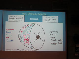 I just want to mention the new interest from String Theory - but which you will hear about on Monday - what little I know - there is a famous conjecture that says that strongly interacting theories in one dimension have a duality with a gravity theory in one higher dimension. The idea is that if you can solve for the motion of particles in a classical gravity theory in one higher dimension will give you the interacting physics of a QFT in the lower dimension. We might all have to learn, or at least remind ourselves about general relativity....
Strongly interacting QFT in D dims <-------> Classical general relativity in at least D+1 dimensions.
Q: Andrey - maybe you should mention the names of Hlubina and Rice
AS: It turns out, that shown by Robert Hlublina and Rice, that you shouldn't do the average over the Fermi surface of the scattering rate, but the scattering time. And when you do this in the clean limit, you get the result that the Fermi liquid T^2 scattering rate dominates. Achim Rosch has shown that in the dirty limit, one can account for non-Fermi liquid behavior at a dirty 2D afm quantum critical point.
Q: Are there any cases where the simple derivation works?
AS: yes is the answer. My favourite is the quantum critical end point of Strontium Ruthenate. Even though the PT to AFM is driven first order by applying a field, you can still at finite field where we get QCP. Does it work there? Well, there is evidence that still more interesting things happen around the quantum critical end-point.
Q: Can you give some simple insight why here you have to take more and more terms, why its failing here, as opposed to BCS theory, where things work out.
AS: BCS is a simple case where you don't have to include fluctuations. Here the problem is that we normally make the assumption that theres a single low-lying mode - but when we deal with metallic systems, we've go other low lying degrees of freedom - could be various types - what we're not able to do is to handle consistently all these low lying modes together. But as a corollary, if you do this in insulators, everything works beautifully. There are cases where quantum criticality does work beautifully, but I was limiting myself to the case of metals, where there are problems.
AChubukov. If I were to answer the question of self consistency. I would answer that formally you can do self-consistency - there is some self-consistency at least at zero level. (We now know there are more subtle problems at higher order - blogger aside - this is a reference to the recent work of Metilsky et al. )

Blogged by Michael Norman and Piers Coleman
Andy is going to do a blackboard talk so let's see how good my eyesight is. The focus will be on ZrZn2, a weak ferromagnet, with the emphasis of how current-current interactions affect metals, and whether the standard Hertz-Millis theory (time dependent Ginzburg-Landau) works or not.
To motivate all of this, let us consider a few cases first. The "strange metal" behavior of cuprates exhibits linear T resistivity over a wide range of temperatures, but the nature of the "ordered" (pseudogap) phase is controversial. CePd2Si2 is an antiferromaget, which is suppressed to zero under pressure. Near the resulting quantum critical point, one sees unconventional superconductivity. Or consider a first order transition (like liquid-gas). At the end of the first order line, one has a second order critical end point, which in principle could be tuned to zero by varying some quantity like field, pressure, or what have you.
Q: What do you mean by critical fluctuations?
AS: Near the ordering phase line, small variations of the order parameter field lead to large responses.

Now to the tutorial. In Landau theory, there is a one to one mapping between non-interacting electrons and fermionic quasiparticles. One can characterize the system by a distribution function, n(E), which varies with momentum, k. The difference from the Fermi function is determined by interactions. This can be determined by a scattering rate, which can be calculated using Fermi's golden rule, taking into account the presence of a filled Fermi sea. One finds that the scattering rate depends on omega^2, where omega is the energy loss. Including temperature, omega^2 changes to omega^2 + (pi*T)^2.
This is a phase space argument. Now, let's assume the scattering potential depends on momentum and energy. Exploiting energy and momentum conservation, one sees that the transferred energy, omega, is restricted to being (T=0) between zero and the energy E of the state, whereas the transferred momentum is restricted to being between omega/vF and 2kF, where vF is the Fermi velocity and kF is the Fermi momentum. The result for the scattering rate (easily derived by power counting) is
1/tau ~ Integral(0 to E) omega domega Integral (omega/vF to 2kF) q^(D-3) dq |V(q,omega)|^2 where V is the scattering potential and D the dimensionality. If V is constant, in D=3, this gives E^2 as before, whereas in D=2, one gets E^2log(E) instead.
If V has structure, then one gets something more interesting. Coulomb scattering looks promising, since V ~ 1/q^2, but screening converts this to 1/(q^2 + qTF^2) where qTF is the Thomas-Fermi wavevector, and the infrared divergence is cutoff.
On the other hand, magnetic scattering is not screened, so this is more promising. Assuming an Amperean potential between currents, j. Using Maxwell equations and Ohm's law, the current-current scattering potential varies as 1/(q^2 - omega^2/c^2 + i*omega*sigma) where sigma is the conductivity. The last term in the denominator is the so-called skin effect. In the clean limit, sigma varies as 1/q. So V^2 goes as 1/q^4 down to q of order omega^(1/3). The result is that 1/tau (D=3) now goes like E instead of E^2. Since 1/tau is a measure of the imaginary part of the self-energy, by Kramers-Kronig, one can show that the real part of the self-energy goes as E*log(E). Therefore, the specific heat coefficient goes as log(T).
But the problem is that the ratio of the Amperean potential to the Coulomb one goes as vF^2/c^2, which is of order 10^(-6). So, although one does indeed find a breakdown of Fermi liquid theory, this only shows up at extremely low temperatures.
Q: This looks like a classical treatment?
AS: Yes and no. One has a Fermi surface, and then treats things in a semi-classical approximation.

Part II. Andy begins with a summary of the first lecture. The blackboard is empty and we are ready for another wonderful blackboard talk. Andy is going to use the results from the last lecture to gain insight into the magnet quantum critical point. Andy says - if I think about an electric current and imagine how it is affected by small angle scattering. A quasiparticle receives a tiny knock, and is now diverted through a small angle - this contributes to the decay rate of the quasiparticle, but it does not affect the transport current very much. (Bloggers aside: We saw this yesterday in Lara Benfatto's talk - this is the effect of the vertex corrections. ) The change in the current is
Delta j = k_F (1-cos (theta)) ~ k_F * (q/k_F)^2
which is reduced by the factor q^2s, so that transport rate is now
current decay rate = Integral omega domega Integral d^D-1 q dq/ q^2 * |V(q,omega)|^2
* additional q^2 term
The q^D-1 cancels with q^2 in D=3, the |V(q,omega)|^2 ~ 1/q^4 at q^2 > omega/q, so the lower limit becomes omega^1/3, so when we do it, we have dq/q^2 from omega^1/3 , which gives 1/omega^1/3 from the q-integral, which gives in the end, with the frequency integral omega^5/3 -> T^5/3. (Blogger's aside - this result is consistent with simple dimensional analysis! AS answers that it is good to see how this works in detail. )
Q: wouldn't you have to do this self-consistently, because the resistivity appears in the damping rate?
AS: Potentially - but it comes back to whether the effective mass should be calculated self-consistently. But the answer seems to be, it doesn't affect anything.
AS asks - can we use these results for U(1) gauge theories, where the coupling constant is much bigger. AS reminds us about the method that was used by Yong Baek in his talk on spin liquids -
fermion = spinon creation * holon (slave boson approach)
Now this introduces a local gauge invariance, and to make this work once the spinons are delocalized, you need a fictitious electromagnetism.
Q: Is this really fictitious - after all it leads to a collective " artificial light ",
AS: I wanted to make the point that it is not conventional Electromagnetism. It is observable, because it will lead to a T^2/3 specific heat. Andy points out that the energy will go like
T^2/3. (Blogger didn't quite catch it all).
Now we discuss Matter close to quantum criticality. The action is written down
S = phi[ r0 + q^2 + |omega|/Gamma(q)]phi + u phi^4
Why do I have a term proportional to omega? Answer - because this is allowing for the physics of damping?
quasiparticle interacts with medium that is almost magnetic, and it sends out modes with a propagator that is the inverse of the quadratic coefficient of S
1 / [r0 + q^2 + |omega|/Gamma(q)]
If you were in an insulator, the damping would be replaced by omega^2. But here we have a metallic environment, the magnon interacts with the Fermi sea which makes particle-hole pairs.
Q: can this be derived?
AS: Yes, but we now know there are some problems with the derivation (non-analytic terms in frequency for example).
So in a system like ZrZn_2 close to criticality, the propagator of the critical magnetization is essentially identical with the current-current fluctuations we talked about this morning, but with a much stronger coupling. And we see a T^5/3 resistivity as expected. Note that the thermal resistivity, which is just governed by the quasiparticle relaxation rate, is still linear in T, as measured by Smith et al in the data shown below.
Q: how do you derive this from the partition function?
AS: Well - we'd like to rewrite the Boltzmann partition function in terms of states that are not eigenstates? Fortunately for me that question was answered long-ago by Feynman, who wanted to use position eigenstates in zero temperature qm. He showed that you could evalue the expectations of
<r | exp[-i H t] r'>
provided you split it up into tiny increments, and then sum over all "histories" {r(t)}. I'm trying to do exactly the same thing here,
< phi | exp[- H beta] |phi> = Sum over the {phi_j} configurations of
< phi | exp [ - H \delta \tau] |phi_1> x ..... x <phi_N-1| exp[-H \delta \tau |phi
I now have imaginary time, and I have to split it up into all trajectories of the magnetization in imaginary time.
Q: I understand all of this, but why does it give rise to the precise form in S that you have shown us?
AS: The answer is that this is the first allowable term in the expansion - why do I have a q^2 - the first that is allowed - you might have though omega^2, but because this is in a damped environment, you can have a |omega|. Actually what we have here is the Lindhardt function - a polarization bubble which has precisely this form.

AS: I kind of lied to you, because ferromagnet is an eigenstate. But when we look at long wavelength modes, (draws a wave) . In the FM, the decay rates are suppressed as the wavelength gets longer and longer, and this gives rise to a damping rate Gamma(q) ~ q. Balistic motion - the amount of time is proportional to the wavelength, which gives tau ~ lambda, 1/tau ~ q. But if it was a dirty ferromagnet, the electrons would diffuse, so now tau ~ lambda ^2, 1/ tau ~ q^2. Final thing I should mention is an antiferromagnet. Now it doesn't depend on the slight variations about the AFM wavelength, so damping rate is constant.
So for an antiferromagnet, the propagator becomes
1 / [ r0 + (Q-q)^2 + |omega|/Gamma_0]
where we expanding the Gamma around the afm wavevector. So now I can change my scattering rate formula, which now becomes centered around Q.
(Q-q) -> qtilde
The denominator has now gone away becomes big Q^2. The q^2/k_F^2 disappears because the scattering is now at large Q, which relaxes the current easily.
Q: Why don't you change the lower limits of integration in momentum?
AS: The upper cutoff isn't really important. Its kind of order (k_F). The lower cutoff is now when p^2 ~ omega, so lower limit is indeed changed to omega^(1/2)
But why is all of this wrong?
Well experimentally - in the FM - almost all of them become first order before we reach the QCP. (Bloggers aside, there is a new Yb system which does have a second order transition, but its more localized)
MnSi is a particularly fascinating case. It also doesn't go quantum critical - weakly first order - and worst, the power law, which is not actually T^5/3, but T^3/2, appears over a wide range of the tuning parameter (presssure) - and nobody understands this.
Theoretical reappraisal.
It turns out that there are additional terms in the LGW action. A more detailed analysis tells us that terms I've left out should affect the answer. Finally - almost everything I've discussed now applies to itinerant systems, where the magnetism is delocalized, but a lot of the crucial experiments are on f-electron systems where the magnetism is very localized, and the itinerant approach I've described here doesn't apply.
A better job of dealing with the FM QCP, there are non-analytic terms, eg in 3D, q^3/2 terms, which leads to fourth order terms that go negative, explaining why the transitions tend to go first order.
The current picture of the FM QCP is as follows:

Now the electrons are coupling to the transverse modes. The early pioneers did not quite take into effect the higher order transverse modes - but if you can gap them out by applying a field, you do get interesting quantum criticality at a metamagnetic QCP.
Puzzles in Heavy Fermion QCP.
Examples include CeCu6-xAu_x
The reason we thought things were fine - that we can ignore the mode-mode coupling terms can be ignored (above the upper critical dimension) - yet there is evidence that the system obeys E/T scaling - a result of something called "naive scaling" - which suggests that the underlying quantum critical point is somehow below its upper critical dimension. There is other evidence that the critical fluctuations are affecting all the Fermi surface - some kind of local quantum criticality.
Another example is YbRh2Si2, which has an incredibly low ordering temperature that is killed off by a tiny magnetic field. Seems to be an additional scale that is collapsing to zero T^* at the QCP. This is one of the great puzzles.
An example of a delocalized heavy fermi liquid, Andy gives UPt3, where the volume of the FS includes the f-moments. The picture thats emerging, is that the QCP could be the merging of Kondo and magnetism - a direct competition between the formation of the heavy fermi liquid and the magnetism. Its not clear that the magnetism and the failure of the heavy fermi liquid need coincide - but they seem to in some systems.

Strongly interacting QFT in D dims <-------> Classical general relativity in at least D+1 dimensions.
Q: Andrey - maybe you should mention the names of Hlubina and Rice
AS: It turns out, that shown by Robert Hlublina and Rice, that you shouldn't do the average over the Fermi surface of the scattering rate, but the scattering time. And when you do this in the clean limit, you get the result that the Fermi liquid T^2 scattering rate dominates. Achim Rosch has shown that in the dirty limit, one can account for non-Fermi liquid behavior at a dirty 2D afm quantum critical point.
Q: Are there any cases where the simple derivation works?
AS: yes is the answer. My favourite is the quantum critical end point of Strontium Ruthenate. Even though the PT to AFM is driven first order by applying a field, you can still at finite field where we get QCP. Does it work there? Well, there is evidence that still more interesting things happen around the quantum critical end-point.
Q: Can you give some simple insight why here you have to take more and more terms, why its failing here, as opposed to BCS theory, where things work out.
AS: BCS is a simple case where you don't have to include fluctuations. Here the problem is that we normally make the assumption that theres a single low-lying mode - but when we deal with metallic systems, we've go other low lying degrees of freedom - could be various types - what we're not able to do is to handle consistently all these low lying modes together. But as a corollary, if you do this in insulators, everything works beautifully. There are cases where quantum criticality does work beautifully, but I was limiting myself to the case of metals, where there are problems.
AChubukov. If I were to answer the question of self consistency. I would answer that formally you can do self-consistency - there is some self-consistency at least at zero level. (We now know there are more subtle problems at higher order - blogger aside - this is a reference to the recent work of Metilsky et al. )
This talk discussed instabilities in Fermi Liquid theory. In this language, what is the instability that drives the Mott transition?
ReplyDeleteTwo questions:
ReplyDelete1) Naive: in the two described ways to get a QCP which one is Quantum spin liquid?
2) Even more naive: At zero temperature the Fermi surface is defined as a locus of the poles of the Green's function G=. If one insist on considering the Maxwell theory one should ask if the quantity is gauge invariant, and G is not. Meaning that FS can not be defined. Is that true? How does this argument breaks for a finite temperature?
What if we consider interaction between electrons mediated by some massless bosons, for example, acoustic phonons, or plasmons in 2D? Can this type of interaction lead to a breakdown of Landau Fermi liquid theory?
ReplyDeleteThe region above (at higher temperatures) the quantum critical point, the so-called quantum critical wedge, is often said to be dominated by critical fluctuations, as defined by Andy in the morning. Presumably this does break down at very high temperatures. What sets the scale where the critical fluctuations are no longer of importance?
ReplyDeleteQ: Is it right to say that there is no quantitative measure of quantum criticality because length/energy scales vanish? How about the rate at which the quasiparticle weight changes, say as a function of tuning, as the QCP is approached?
ReplyDeleteQ: The action as written down in the lecture had an anisotropy between space and time: what's a main difference between a QCP that's space-time isotropic and this?
Vipin